Gradient Ascent, Global Maximum, and Complexity
In my last post, I talked about the determination of origin (point A), the point from which you begin your journey. I briefly highlighted why I think it is important to define some point as the origin of your endeavours, for in absence of such a point, how do you even begin to place yourself on a map of possibilities. I then moved on to talk about defining point B, the point that you want to go towards and one that, to a great extent, captures all the things that you currently are not but want to be. On this mental map of potential, point B is higher than point A.
Now, for most complex games it isn’t necessarily evident to a beginner (or even an expert) what the highest point in the game is. For example, sports athletes continually surpass previously set records only for those to be broken once again. As such, our collective comprehension of maximum potential continuously evolves. In this context,
-
How should a player go about choosing point B?
-
Once chosen, is there a particular strategy that a player can follow to move towards point B?
-
If so, how does the player verify that s/he is moving towards point B?
Before we move further with our investigation, I do want to state that the below analysis is not a “technical” one per se. In some ways it’s a playful digression from the purely philosophical realm, drawing insights from the application of techniques from a more quantitative discipline. It goes without saying that both, quantitative and qualitative, models are but restricted representations of reality and should be viewed as such.
Ok then, back to the issue at hand. Once we have defined the origin, point A, and agree that we want to move to a higher point, point B, we need a strategy to move forward. For this, I’ll borrow an algorithm called “gradient descent” from statistics.
“A gradient descent algorithm is a method used to minimize a given objective function by iteratively adjusting the algorithm parameters in the direction of the steepest descent of the function. It is one of the most widely used optimization algorithms.”
Here’s how it works:
-
Initialization: It starts with an initial set of parameter values and starting point (our origin/point A).
-
Gradient Calculation: It calculates the gradient of the objective function (think of this as the surface on which we’re playing our game) with respect to the parameters.
-
Parameter Update: It updates the parameters in the opposite direction of the gradient, scaled by a chosen step size (learning rate).
-
Convergence Check: It repeats steps 2 and 3 until convergence criteria are met, such as reaching a maximum number of iterations or a sufficiently small change in the objective function.
For those of you who want to dig into this further, I found a really good description of the algorithm here.
As stated above, gradient descent is a nice and simple algorithm that is used to find the function minimum using the slope/gradient of the given function. As inputs, it requires the starting point, the gradient of a function at the given point, and defined parameters - learning rate and number of steps (epochs) - for which the user wants the algorithm to run. Gradient descent algorithm iteratively calculates the next position using slope at the current position, scales it by a learning rate, and subtracts obtained value from the current position (makes a step). It subtracts the value because we want to minimise the function.
Now if gradient descent algorithm can be used to find the minimum of a function, we should be able to flip the algorithm to the find the maximum of the function as well. All we really need for this is to tweak one step in the algorithm where instead of moving in opposite direction of the gradient, we move in the direction of the gradient. In other words, to take the next step in point (3) above we add the scaled gradient to our current position.
Below is the python code that takes the initial point as input and runs the algorithm to output the next point.
def gradient_ascent(x_start, y_start, learning_rate, epochs, grad):
    x = x_start
    y = y_start
    for _ in range(epochs):
        # grad is a function that calculates the respective gradients
        grad_x, grad_y = grad(x, y)
        x += learning_rate * grad_x  # move in the direction of the gradient
        y += learning_rate * grad_y
    return x, y
For my experiment,
I’ll use two bi-variate functions (no particular reason beyond that I want to plot some nice 3D graphs for better visualisation of the surface) of the form that have multiple minima and maxima.
I’ll assume that the 3D surface is a constrained representation of the game where our player goes from point A to point B.
A player will start at an initial point (point A) with the aim of reaching the global maximum (point B). Note that our player neither knows what the entire surface looks like nor what the global maximum is.
A player’s initial point (point A) is determined randomly. I’ll draw the x and y coordinates from a normal distribution. This seems reasonable to me as in any game one seldom has the agency to dictate the initial allocation of resources bestowed upon them.
The player will use gradient ascent algorithm to try and find the global maximum.
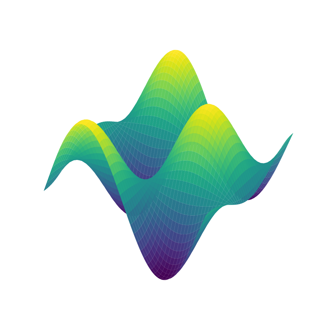
We’re now set-up. Let’s begin with our first function below (see cover image to visualise the function).
# Define the first function
def f1(x, y):
    return np.sin(x/3) * np.cos(y/3)
I chose the first function primarily because of its sinusoidal symmetry. In simple words, as you can see (in the cover image above and image immediately below), the function has some nice symmetric features in presenting a landscape with equal minimum and maximum points and -1 and +1, respectively. To me, this is the simplest approximation of a game that one might play because of two reasons: (i) the surface is smooth with function min and max that do not go outside a bounded range (ii) the symmetry can be thought of as all players striving for the same (unknown) point B. Reality of course can be more complex with different players seeking and optimising for different points.
Let’s run our first simulation with learning rate = 0.01 and epochs = 1000.
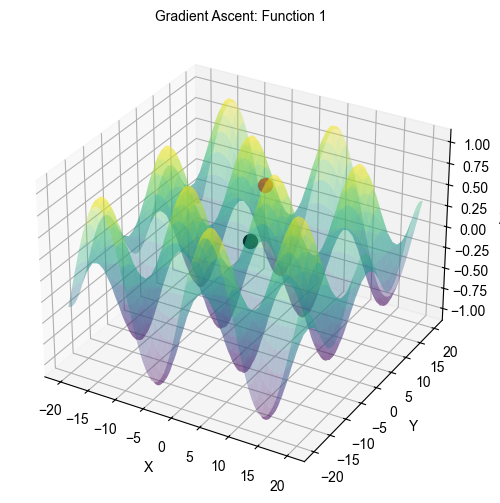
Maximum point reached: x = 3.07, y = 0.06, z = 0.85
Vertical distance travelled: 0.70
In the picture above, the black dot is our point A and the red dot represents where the player finally ends up after the algorithm runs its course. Note that while the red dot is not necessarily point B (global maximum), it is still higher than our starting point. Some observations at this juncture below.
-
Using the algorithm, we’ve already devised one method of going from point A towards point B.
-
Starting from point A, we assumed that the player doesn’t know what the function maximum is. Per the algorithm, the player starts moving directly in the direction of the gradient, which is the direction of the steepest ascent. You can check out why the gradient is the direction of steepest ascent in this great video from Khan Academy here. In my opinion, this is already quite a powerful insight. When you begin a game and aspire towards a higher point, the optimal course of action entails navigating towards the direction of greatest ascent. In a philosophical context, this concept mirrors the imperative of confronting one’s deepest apprehensions and pressing forward towards endeavours that we know we must engage with but find uncomfortable and have postponed for far too long.
-
Note that in the code for gradient ascent algorithm step size is defined as learning rate * gradient. Given that the learning rate is set to 0.01, the player is taking iterative steps towards an unknown maximum. At the end of the first step, the algorithm repeats but there is something different at the new (updated) point. Given that this function is concave (ignore saddle points), intuitively the slope is getting flatter and flatter as we get closer to the maximum. This means that with each passing step, the player’s step size is actually getting smaller, implying that as the player is closing in on the maximum point the player is taking smaller steps (astute readers will already see how the algorithm reaches its goal; at the maximum point, gradient/slope will be near zero resulting in an infinitesimally small step size). Philosophically, this presents a conundrum. Intuitively, one might surmise that as the gradient flattens, one should accelerate progress by taking larger steps. However, the algorithm suggests a contrasting approach: caution and restraint are warranted as the summit is neared, lest one overshoots the maximum. Maybe the insight here is that, given the decreasing room for error near the maximum, our player needs to be more cautious at the top compared to the bottom.
-
As previously discussed, the initial point is a random draw from a normal distribution. This means that our player may get lucky and land up right next to the maximum. Assuming that the player is constrained by computational resources (and we always are!), it is not necessary that all players will reach the maximum point within the defined number of steps. As such, its seems appropriate that we judge the player for the actual distance travelled rather than if the player reached the maximum point or not.
As a next step, I ran 1000 simulations of the above set-up. Below is a histogram of the (normalised) vertical distance travelled.
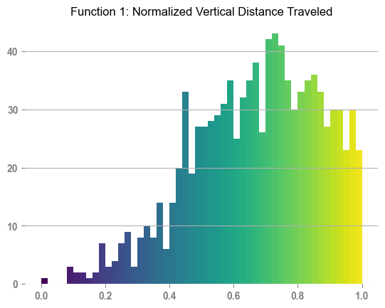
Mean: 0.67
Std: 0.20
A notable trend emerges: a substantial proportion of players exhibit significant progress along the ascent trajectory. The average distance traveled underscores this observation, indicating a commendable level of advancement achieved by the majority of participants. Furthermore, a notable concentration of players is observed on the right end of the distribution.
Great, let’s raise the complexity by introducing our second function: Ackley function[1]. The Ackley function is a widely studied mathematical function commonly used in optimisation and computational experiments. You can read more about this here. We will, of course, multiply the function by -1 to get a global maximum instead of a global minimum. In its bivariate form, the functions looks like the one below:
#defining the Ackley function
def f2(x, y):
    a = 20
    b = 0.2
    c = 2 * np.pi
    term1 = -a * np.exp(-b * np.sqrt(0.5 * (x**2 + y**2)))
    term2 = -np.exp(0.5 * (np.cos(c*x) + np.cos(c*y)))
    return (term1 + term2 + a + np.exp(1))*-1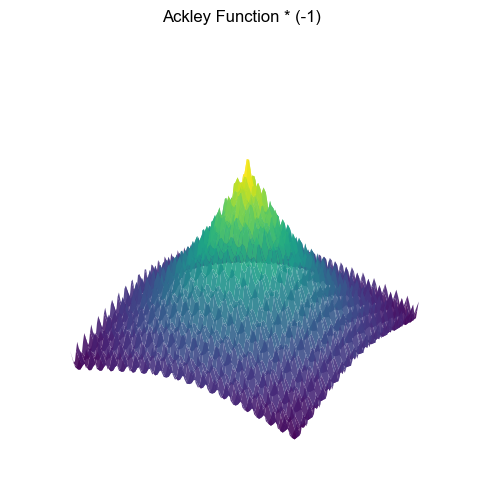
This time, running the same algorithm presents a very different view of the distance travelled by our players.
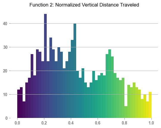
Mean: 0.45
Std: 0.26
Some further observations below:
-
As the complexity of the function has increased, i.e., we now have multiple local maxima with a global maximum, we are starting to see a divergence in player performance. With the same starting distribution, there are now fewer players who find themselves in the right end of the distribution. Further, the computational time taken the run 1000 simulations has gone up significantly. Where the first set of the simulations took 2.0s, this set of simulations has taken 45m 43s to run.
-
In our exploration of Function 1, we discerned that the maximum value of the function is bounded at +1. Conceptually, Function 1 embodies the structure of a single level within a game, where players commence their journey with a clear objective: to attain the maximum point within a level. The narrative evolves with the introduction of the Ackley function, which introduces a dynamic interplay of multiple local maxima and a global maximum.
-
This paradigm shift prompts a reimagining of the game: each local maximum here can be viewed as serving a distinct level within the game, with players ascending to the “next level” upon surpassing each successive peak. In essence, the Ackley function encapsulates the entirety of the game with multiple levels!
- The very first insight that I draw from this is that just because a player’s algorithm generally works for one level (in our case, function 1), it isn’t obvious that it’ll continue to work for higher and more complex levels.
- Secondly, if a player finds that s/he is expending way more resources (reflected by increased computational time) to reach the same vertical distance, it may potentially be a signal that the player has “levelled up”? If so, I think it helps us answer the question whether the player is making progress or not.
- Lastly, assuming that the player doesn’t want to change the algorithm, I think that the player is justified to stop and ask if it even makes sense to continue pushing forward to reach for the global maximum. This decision-making process aligns with the principles of the Pareto principle, wherein players weigh the potential gains of pushing further against the increased costs and diminishing returns associated with higher levels of attainment. At this point, it may be more prudent to start a different game altogether?
This discourse has been extensive, and I trust that you found it enriching and thought-provoking. For those inclined to delve deeper into the subject matter, you can find the underlying Python script on GitHub.
Once again, it is worth re-mentioning that the insights presented here are contingent upon the specific functions and initial distributions chosen for analysis. Therefore, it is essential to acknowledge that this discussion does not purport to be a “technical” analysis. Do let me know if you find something different in our own exploration.
Notes and References:
[1] Ackley, D. H. (1987) “A connectionist machine for genetic hillclimbing”, Kluwer Academic Publishers, Boston MA. p. 13-14